Multiclass TF
Optional Lab - Multi-class Classification
1.1 Goals
In this lab, you will explore an example of multi-class classification using neural networks.

1.2 Tools
You will use some plotting routines. These are stored in lab_utils_multiclass_TF.py in this directory.
import numpy as np
import matplotlib.pyplot as plt
%matplotlib widget
from sklearn.datasets import make_blobs
import tensorflow as tf
from tensorflow.keras.models import Sequential
from tensorflow.keras.layers import Dense
np.set_printoptions(precision=2)
from lab_utils_multiclass_TF import *
import logging
logging.getLogger("tensorflow").setLevel(logging.ERROR)
tf.autograph.set_verbosity(0)
2.0 Multi-class Classification
Neural Networks are often used to classify data. Examples are neural networks:
- take in photos and classify subjects in the photos as {dog,cat,horse,other}
- take in a sentence and classify the 'parts of speech' of its elements: {noun, verb, adjective etc..}
A network of this type will have multiple units in its final layer. Each output is associated with a category. When an input example is applied to the network, the output with the highest value is the category predicted. If the output is applied to a softmax function, the output of the softmax will provide probabilities of the input being in each category.
In this lab you will see an example of building a multiclass network in Tensorflow. We will then take a look at how the neural network makes its predictions.
Let's start by creating a four-class data set.
2.1 Prepare and visualize our data
We will use Scikit-Learn make_blobs function to make a training data set with 4 categories as shown in the plot below.
# make 4-class dataset for classification
classes = 4
m = 100
centers = [[-5, 2], [-2, -2], [1, 2], [5, -2]]
std = 1.0
X_train, y_train = make_blobs(n_samples=m, centers=centers, cluster_std=std,random_state=30)
print(X_train.shape)
(100, 2)
plt_mc(X_train,y_train,classes, centers, std=std)

Each dot represents a training example. The axis (x0,x1) are the inputs and the color represents the class the example is associated with. Once trained, the model will be presented with a new example, (x0,x1), and will predict the class.
While generated, this data set is representative of many real-world classification problems. There are several input features (x0,...,xn) and several output categories. The model is trained to use the input features to predict the correct output category.
# show classes in data set
print(f"unique classes {np.unique(y_train)}")
# show how classes are represented
print(f"class representation {y_train[:10]}")
# show shapes of our dataset
print(f"shape of X_train: {X_train.shape}, shape of y_train: {y_train.shape}")
unique classes [0 1 2 3]
class representation [3 3 3 0 3 3 3 3 2 0]
shape of X_train: (100, 2), shape of y_train: (100,)
2.2 Model
 This lab will use a 2-layer network as shown.
Unlike the binary classification networks, this network has four outputs, one for each class. Given an input example, the output with the highest value is the predicted class of the input.
This lab will use a 2-layer network as shown.
Unlike the binary classification networks, this network has four outputs, one for each class. Given an input example, the output with the highest value is the predicted class of the input.
Below is an example of how to construct this network in Tensorflow. Notice the output layer uses a linear rather than a softmax activation. While it is possible to include the softmax in the output layer, it is more numerically stable if linear outputs are passed to the loss function during training. If the model is used to predict probabilities, the softmax can be applied at that point.
tf.random.set_seed(1234)  # applied to achieve consistent results
model = Sequential(
    [
        Dense(2, activation = 'relu',   name = "L1"),
        Dense(4, activation = 'linear', name = "L2")
    ]
)
The statements below compile and train the network. Setting from_logits=True as an argument to the loss function specifies that the output activation was linear rather than a softmax.
model.compile(
    loss=tf.keras.losses.SparseCategoricalCrossentropy(from_logits=True),
    optimizer=tf.keras.optimizers.Adam(0.01),
)

model.fit(
    X_train,y_train,
    epochs=200
)
Epoch 1/200
4/4 ━━━━━━━━━━━━━━━━━━━━ 1s 10ms/step - loss: 2.7849
Epoch 2/200
4/4 ━━━━━━━━━━━━━━━━━━━━ 0s 6ms/step - loss: 2.5192
Epoch 3/200
4/4 ━━━━━━━━━━━━━━━━━━━━ 0s 8ms/step - loss: 2.2868
Epoch 4/200
4/4 ━━━━━━━━━━━━━━━━━━━━ 0s 6ms/step - loss: 2.0815
Epoch 5/200
4/4 ━━━━━━━━━━━━━━━━━━━━ 0s 5ms/step - loss: 1.9020
Epoch 6/200
4/4 ━━━━━━━━━━━━━━━━━━━━ 0s 6ms/step - loss: 1.7498
Epoch 7/200
4/4 ━━━━━━━━━━━━━━━━━━━━ 0s 7ms/step - loss: 1.6209
Epoch 8/200
4/4 ━━━━━━━━━━━━━━━━━━━━ 0s 6ms/step - loss: 1.5123
Epoch 9/200
4/4 ━━━━━━━━━━━━━━━━━━━━ 0s 7ms/step - loss: 1.4221
Epoch 10/200
4/4 ━━━━━━━━━━━━━━━━━━━━ 0s 8ms/step - loss: 1.3488
Epoch 11/200
4/4 ━━━━━━━━━━━━━━━━━━━━ 0s 7ms/step - loss: 1.2882
Epoch 12/200
4/4 ━━━━━━━━━━━━━━━━━━━━ 0s 6ms/step - loss: 1.2367
Epoch 13/200
4/4 ━━━━━━━━━━━━━━━━━━━━ 0s 7ms/step - loss: 1.1925
Epoch 14/200
4/4 ━━━━━━━━━━━━━━━━━━━━ 0s 6ms/step - loss: 1.1554
Epoch 15/200
4/4 ━━━━━━━━━━━━━━━━━━━━ 0s 6ms/step - loss: 1.1239
Epoch 16/200
4/4 ━━━━━━━━━━━━━━━━━━━━ 0s 7ms/step - loss: 1.0964
Epoch 17/200
4/4 ━━━━━━━━━━━━━━━━━━━━ 0s 7ms/step - loss: 1.0723
Epoch 18/200
4/4 ━━━━━━━━━━━━━━━━━━━━ 0s 6ms/step - loss: 1.0505
Epoch 19/200
4/4 ━━━━━━━━━━━━━━━━━━━━ 0s 6ms/step - loss: 1.0307
Epoch 20/200
4/4 ━━━━━━━━━━━━━━━━━━━━ 0s 7ms/step - loss: 1.0123
Epoch 21/200
4/4 ━━━━━━━━━━━━━━━━━━━━ 0s 8ms/step - loss: 0.9948
Epoch 22/200
4/4 ━━━━━━━━━━━━━━━━━━━━ 0s 6ms/step - loss: 0.9780
Epoch 23/200
4/4 ━━━━━━━━━━━━━━━━━━━━ 0s 7ms/step - loss: 0.9620
Epoch 24/200
4/4 ━━━━━━━━━━━━━━━━━━━━ 0s 6ms/step - loss: 0.9462
Epoch 25/200
4/4 ━━━━━━━━━━━━━━━━━━━━ 0s 6ms/step - loss: 0.9304
Epoch 26/200
4/4 ━━━━━━━━━━━━━━━━━━━━ 0s 7ms/step - loss: 0.9148
Epoch 27/200
4/4 ━━━━━━━━━━━━━━━━━━━━ 0s 6ms/step - loss: 0.8994
Epoch 28/200
4/4 ━━━━━━━━━━━━━━━━━━━━ 0s 6ms/step - loss: 0.8842
Epoch 29/200
4/4 ━━━━━━━━━━━━━━━━━━━━ 0s 6ms/step - loss: 0.8694
Epoch 30/200
4/4 ━━━━━━━━━━━━━━━━━━━━ 0s 6ms/step - loss: 0.8550
Epoch 31/200
4/4 ━━━━━━━━━━━━━━━━━━━━ 0s 7ms/step - loss: 0.8408
Epoch 32/200
4/4 ━━━━━━━━━━━━━━━━━━━━ 0s 7ms/step - loss: 0.8269
Epoch 33/200
4/4 ━━━━━━━━━━━━━━━━━━━━ 0s 6ms/step - loss: 0.8134
Epoch 34/200
4/4 ━━━━━━━━━━━━━━━━━━━━ 0s 8ms/step - loss: 0.8005
Epoch 35/200
4/4 ━━━━━━━━━━━━━━━━━━━━ 0s 7ms/step - loss: 0.7880
Epoch 36/200
4/4 ━━━━━━━━━━━━━━━━━━━━ 0s 8ms/step - loss: 0.7762
Epoch 37/200
4/4 ━━━━━━━━━━━━━━━━━━━━ 0s 8ms/step - loss: 0.7649
Epoch 38/200
4/4 ━━━━━━━━━━━━━━━━━━━━ 0s 6ms/step - loss: 0.7540
Epoch 39/200
4/4 ━━━━━━━━━━━━━━━━━━━━ 0s 8ms/step - loss: 0.7434
Epoch 40/200
4/4 ━━━━━━━━━━━━━━━━━━━━ 0s 8ms/step - loss: 0.7332
Epoch 41/200
4/4 ━━━━━━━━━━━━━━━━━━━━ 0s 6ms/step - loss: 0.7232
Epoch 42/200
4/4 ━━━━━━━━━━━━━━━━━━━━ 0s 7ms/step - loss: 0.7135
Epoch 43/200
4/4 ━━━━━━━━━━━━━━━━━━━━ 0s 6ms/step - loss: 0.7041
Epoch 44/200
4/4 ━━━━━━━━━━━━━━━━━━━━ 0s 6ms/step - loss: 0.6950
Epoch 45/200
4/4 ━━━━━━━━━━━━━━━━━━━━ 0s 8ms/step - loss: 0.6861
Epoch 46/200
4/4 ━━━━━━━━━━━━━━━━━━━━ 0s 7ms/step - loss: 0.6774
Epoch 47/200
4/4 ━━━━━━━━━━━━━━━━━━━━ 0s 8ms/step - loss: 0.6690
Epoch 48/200
4/4 ━━━━━━━━━━━━━━━━━━━━ 0s 7ms/step - loss: 0.6609
Epoch 49/200
4/4 ━━━━━━━━━━━━━━━━━━━━ 0s 8ms/step - loss: 0.6530
Epoch 50/200
4/4 ━━━━━━━━━━━━━━━━━━━━ 0s 6ms/step - loss: 0.6454
Epoch 51/200
4/4 ━━━━━━━━━━━━━━━━━━━━ 0s 6ms/step - loss: 0.6379
Epoch 52/200
4/4 ━━━━━━━━━━━━━━━━━━━━ 0s 7ms/step - loss: 0.6307
Epoch 53/200
4/4 ━━━━━━━━━━━━━━━━━━━━ 0s 6ms/step - loss: 0.6237
Epoch 54/200
4/4 ━━━━━━━━━━━━━━━━━━━━ 0s 6ms/step - loss: 0.6168
Epoch 55/200
4/4 ━━━━━━━━━━━━━━━━━━━━ 0s 6ms/step - loss: 0.6100
Epoch 56/200
4/4 ━━━━━━━━━━━━━━━━━━━━ 0s 6ms/step - loss: 0.6033
Epoch 57/200
4/4 ━━━━━━━━━━━━━━━━━━━━ 0s 8ms/step - loss: 0.5968
Epoch 58/200
4/4 ━━━━━━━━━━━━━━━━━━━━ 0s 6ms/step - loss: 0.5904
Epoch 59/200
4/4 ━━━━━━━━━━━━━━━━━━━━ 0s 6ms/step - loss: 0.5840
Epoch 60/200
4/4 ━━━━━━━━━━━━━━━━━━━━ 0s 6ms/step - loss: 0.5778
Epoch 61/200
4/4 ━━━━━━━━━━━━━━━━━━━━ 0s 7ms/step - loss: 0.5717
Epoch 62/200
4/4 ━━━━━━━━━━━━━━━━━━━━ 0s 7ms/step - loss: 0.5657
Epoch 63/200
4/4 ━━━━━━━━━━━━━━━━━━━━ 0s 6ms/step - loss: 0.5598
Epoch 64/200
4/4 ━━━━━━━━━━━━━━━━━━━━ 0s 7ms/step - loss: 0.5540
Epoch 65/200
4/4 ━━━━━━━━━━━━━━━━━━━━ 0s 6ms/step - loss: 0.5483
Epoch 66/200
4/4 ━━━━━━━━━━━━━━━━━━━━ 0s 6ms/step - loss: 0.5427
Epoch 67/200
4/4 ━━━━━━━━━━━━━━━━━━━━ 0s 6ms/step - loss: 0.5371
Epoch 68/200
4/4 ━━━━━━━━━━━━━━━━━━━━ 0s 8ms/step - loss: 0.5315
Epoch 69/200
4/4 ━━━━━━━━━━━━━━━━━━━━ 0s 7ms/step - loss: 0.5260
Epoch 70/200
4/4 ━━━━━━━━━━━━━━━━━━━━ 0s 8ms/step - loss: 0.5204
Epoch 71/200
4/4 ━━━━━━━━━━━━━━━━━━━━ 0s 8ms/step - loss: 0.5145
Epoch 72/200
4/4 ━━━━━━━━━━━━━━━━━━━━ 0s 6ms/step - loss: 0.5083
Epoch 73/200
4/4 ━━━━━━━━━━━━━━━━━━━━ 0s 7ms/step - loss: 0.5020
Epoch 74/200
4/4 ━━━━━━━━━━━━━━━━━━━━ 0s 6ms/step - loss: 0.4951
Epoch 75/200
4/4 ━━━━━━━━━━━━━━━━━━━━ 0s 6ms/step - loss: 0.4879
Epoch 76/200
4/4 ━━━━━━━━━━━━━━━━━━━━ 0s 6ms/step - loss: 0.4808
Epoch 77/200
4/4 ━━━━━━━━━━━━━━━━━━━━ 0s 6ms/step - loss: 0.4738
Epoch 78/200
4/4 ━━━━━━━━━━━━━━━━━━━━ 0s 6ms/step - loss: 0.4669
Epoch 79/200
4/4 ━━━━━━━━━━━━━━━━━━━━ 0s 7ms/step - loss: 0.4602
Epoch 80/200
4/4 ━━━━━━━━━━━━━━━━━━━━ 0s 8ms/step - loss: 0.4536
Epoch 81/200
4/4 ━━━━━━━━━━━━━━━━━━━━ 0s 8ms/step - loss: 0.4470
Epoch 82/200
4/4 ━━━━━━━━━━━━━━━━━━━━ 0s 6ms/step - loss: 0.4401
Epoch 83/200
4/4 ━━━━━━━━━━━━━━━━━━━━ 0s 7ms/step - loss: 0.4330
Epoch 84/200
4/4 ━━━━━━━━━━━━━━━━━━━━ 0s 6ms/step - loss: 0.4260
Epoch 85/200
4/4 ━━━━━━━━━━━━━━━━━━━━ 0s 6ms/step - loss: 0.4192
Epoch 86/200
4/4 ━━━━━━━━━━━━━━━━━━━━ 0s 6ms/step - loss: 0.4127
Epoch 87/200
4/4 ━━━━━━━━━━━━━━━━━━━━ 0s 6ms/step - loss: 0.4061
Epoch 88/200
4/4 ━━━━━━━━━━━━━━━━━━━━ 0s 6ms/step - loss: 0.3994
Epoch 89/200
4/4 ━━━━━━━━━━━━━━━━━━━━ 0s 6ms/step - loss: 0.3929
Epoch 90/200
4/4 ━━━━━━━━━━━━━━━━━━━━ 0s 6ms/step - loss: 0.3866
Epoch 91/200
4/4 ━━━━━━━━━━━━━━━━━━━━ 0s 6ms/step - loss: 0.3804
Epoch 92/200
4/4 ━━━━━━━━━━━━━━━━━━━━ 0s 7ms/step - loss: 0.3742
Epoch 93/200
4/4 ━━━━━━━━━━━━━━━━━━━━ 0s 7ms/step - loss: 0.3681
Epoch 94/200
4/4 ━━━━━━━━━━━━━━━━━━━━ 0s 6ms/step - loss: 0.3615
Epoch 95/200
4/4 ━━━━━━━━━━━━━━━━━━━━ 0s 7ms/step - loss: 0.3549
Epoch 96/200
4/4 ━━━━━━━━━━━━━━━━━━━━ 0s 6ms/step - loss: 0.3485
Epoch 97/200
4/4 ━━━━━━━━━━━━━━━━━━━━ 0s 6ms/step - loss: 0.3424
Epoch 98/200
4/4 ━━━━━━━━━━━━━━━━━━━━ 0s 7ms/step - loss: 0.3365
Epoch 99/200
4/4 ━━━━━━━━━━━━━━━━━━━━ 0s 6ms/step - loss: 0.3309
Epoch 100/200
4/4 ━━━━━━━━━━━━━━━━━━━━ 0s 7ms/step - loss: 0.3255
Epoch 101/200
4/4 ━━━━━━━━━━━━━━━━━━━━ 0s 6ms/step - loss: 0.3204
Epoch 102/200
4/4 ━━━━━━━━━━━━━━━━━━━━ 0s 6ms/step - loss: 0.3151
Epoch 103/200
4/4 ━━━━━━━━━━━━━━━━━━━━ 0s 7ms/step - loss: 0.3094
Epoch 104/200
4/4 ━━━━━━━━━━━━━━━━━━━━ 0s 7ms/step - loss: 0.3037
Epoch 105/200
4/4 ━━━━━━━━━━━━━━━━━━━━ 0s 7ms/step - loss: 0.2982
Epoch 106/200
4/4 ━━━━━━━━━━━━━━━━━━━━ 0s 6ms/step - loss: 0.2928
Epoch 107/200
4/4 ━━━━━━━━━━━━━━━━━━━━ 0s 7ms/step - loss: 0.2876
Epoch 108/200
4/4 ━━━━━━━━━━━━━━━━━━━━ 0s 6ms/step - loss: 0.2826
Epoch 109/200
4/4 ━━━━━━━━━━━━━━━━━━━━ 0s 7ms/step - loss: 0.2778
Epoch 110/200
4/4 ━━━━━━━━━━━━━━━━━━━━ 0s 6ms/step - loss: 0.2733
Epoch 111/200
4/4 ━━━━━━━━━━━━━━━━━━━━ 0s 6ms/step - loss: 0.2689
Epoch 112/200
4/4 ━━━━━━━━━━━━━━━━━━━━ 0s 7ms/step - loss: 0.2646
Epoch 113/200
4/4 ━━━━━━━━━━━━━━━━━━━━ 0s 7ms/step - loss: 0.2606
Epoch 114/200
4/4 ━━━━━━━━━━━━━━━━━━━━ 0s 6ms/step - loss: 0.2567
Epoch 115/200
4/4 ━━━━━━━━━━━━━━━━━━━━ 0s 6ms/step - loss: 0.2528
Epoch 116/200
4/4 ━━━━━━━━━━━━━━━━━━━━ 0s 6ms/step - loss: 0.2485
Epoch 117/200
4/4 ━━━━━━━━━━━━━━━━━━━━ 0s 6ms/step - loss: 0.2443
Epoch 118/200
4/4 ━━━━━━━━━━━━━━━━━━━━ 0s 6ms/step - loss: 0.2402
Epoch 119/200
4/4 ━━━━━━━━━━━━━━━━━━━━ 0s 6ms/step - loss: 0.2362
Epoch 120/200
4/4 ━━━━━━━━━━━━━━━━━━━━ 0s 7ms/step - loss: 0.2324
Epoch 121/200
4/4 ━━━━━━━━━━━━━━━━━━━━ 0s 7ms/step - loss: 0.2288
Epoch 122/200
4/4 ━━━━━━━━━━━━━━━━━━━━ 0s 6ms/step - loss: 0.2253
Epoch 123/200
4/4 ━━━━━━━━━━━━━━━━━━━━ 0s 6ms/step - loss: 0.2219
Epoch 124/200
4/4 ━━━━━━━━━━━━━━━━━━━━ 0s 9ms/step - loss: 0.2187
Epoch 125/200
4/4 ━━━━━━━━━━━━━━━━━━━━ 0s 6ms/step - loss: 0.2155
Epoch 126/200
4/4 ━━━━━━━━━━━━━━━━━━━━ 0s 8ms/step - loss: 0.2124
Epoch 127/200
4/4 ━━━━━━━━━━━━━━━━━━━━ 0s 6ms/step - loss: 0.2094
Epoch 128/200
4/4 ━━━━━━━━━━━━━━━━━━━━ 0s 7ms/step - loss: 0.2066
Epoch 129/200
4/4 ━━━━━━━━━━━━━━━━━━━━ 0s 7ms/step - loss: 0.2038
Epoch 130/200
4/4 ━━━━━━━━━━━━━━━━━━━━ 0s 7ms/step - loss: 0.2011
Epoch 131/200
4/4 ━━━━━━━━━━━━━━━━━━━━ 0s 6ms/step - loss: 0.1986
Epoch 132/200
4/4 ━━━━━━━━━━━━━━━━━━━━ 0s 7ms/step - loss: 0.1961
Epoch 133/200
4/4 ━━━━━━━━━━━━━━━━━━━━ 0s 6ms/step - loss: 0.1938
Epoch 134/200
4/4 ━━━━━━━━━━━━━━━━━━━━ 0s 6ms/step - loss: 0.1915
Epoch 135/200
4/4 ━━━━━━━━━━━━━━━━━━━━ 0s 8ms/step - loss: 0.1893
Epoch 136/200
4/4 ━━━━━━━━━━━━━━━━━━━━ 0s 8ms/step - loss: 0.1872
Epoch 137/200
4/4 ━━━━━━━━━━━━━━━━━━━━ 0s 8ms/step - loss: 0.1849
Epoch 138/200
4/4 ━━━━━━━━━━━━━━━━━━━━ 0s 6ms/step - loss: 0.1822
Epoch 139/200
4/4 ━━━━━━━━━━━━━━━━━━━━ 0s 7ms/step - loss: 0.1793
Epoch 140/200
4/4 ━━━━━━━━━━━━━━━━━━━━ 0s 6ms/step - loss: 0.1763
Epoch 141/200
4/4 ━━━━━━━━━━━━━━━━━━━━ 0s 7ms/step - loss: 0.1734
Epoch 142/200
4/4 ━━━━━━━━━━━━━━━━━━━━ 0s 7ms/step - loss: 0.1705
Epoch 143/200
4/4 ━━━━━━━━━━━━━━━━━━━━ 0s 7ms/step - loss: 0.1678
Epoch 144/200
4/4 ━━━━━━━━━━━━━━━━━━━━ 0s 6ms/step - loss: 0.1651
Epoch 145/200
4/4 ━━━━━━━━━━━━━━━━━━━━ 0s 6ms/step - loss: 0.1627
Epoch 146/200
4/4 ━━━━━━━━━━━━━━━━━━━━ 0s 6ms/step - loss: 0.1603
Epoch 147/200
4/4 ━━━━━━━━━━━━━━━━━━━━ 0s 6ms/step - loss: 0.1581
Epoch 148/200
4/4 ━━━━━━━━━━━━━━━━━━━━ 0s 7ms/step - loss: 0.1559
Epoch 149/200
4/4 ━━━━━━━━━━━━━━━━━━━━ 0s 6ms/step - loss: 0.1539
Epoch 150/200
4/4 ━━━━━━━━━━━━━━━━━━━━ 0s 6ms/step - loss: 0.1519
Epoch 151/200
4/4 ━━━━━━━━━━━━━━━━━━━━ 0s 8ms/step - loss: 0.1501
Epoch 152/200
4/4 ━━━━━━━━━━━━━━━━━━━━ 0s 6ms/step - loss: 0.1482
Epoch 153/200
4/4 ━━━━━━━━━━━━━━━━━━━━ 0s 7ms/step - loss: 0.1461
Epoch 154/200
4/4 ━━━━━━━━━━━━━━━━━━━━ 0s 7ms/step - loss: 0.1439
Epoch 155/200
4/4 ━━━━━━━━━━━━━━━━━━━━ 0s 7ms/step - loss: 0.1416
Epoch 156/200
4/4 ━━━━━━━━━━━━━━━━━━━━ 0s 6ms/step - loss: 0.1391
Epoch 157/200
4/4 ━━━━━━━━━━━━━━━━━━━━ 0s 7ms/step - loss: 0.1365
Epoch 158/200
4/4 ━━━━━━━━━━━━━━━━━━━━ 0s 6ms/step - loss: 0.1338
Epoch 159/200
4/4 ━━━━━━━━━━━━━━━━━━━━ 0s 7ms/step - loss: 0.1312
Epoch 160/200
4/4 ━━━━━━━━━━━━━━━━━━━━ 0s 7ms/step - loss: 0.1283
Epoch 161/200
4/4 ━━━━━━━━━━━━━━━━━━━━ 0s 7ms/step - loss: 0.1253
Epoch 162/200
4/4 ━━━━━━━━━━━━━━━━━━━━ 0s 7ms/step - loss: 0.1223
Epoch 163/200
4/4 ━━━━━━━━━━━━━━━━━━━━ 0s 6ms/step - loss: 0.1193
Epoch 164/200
4/4 ━━━━━━━━━━━━━━━━━━━━ 0s 7ms/step - loss: 0.1163
Epoch 165/200
4/4 ━━━━━━━━━━━━━━━━━━━━ 0s 6ms/step - loss: 0.1134
Epoch 166/200
4/4 ━━━━━━━━━━━━━━━━━━━━ 0s 7ms/step - loss: 0.1105
Epoch 167/200
4/4 ━━━━━━━━━━━━━━━━━━━━ 0s 7ms/step - loss: 0.1077
Epoch 168/200
4/4 ━━━━━━━━━━━━━━━━━━━━ 0s 8ms/step - loss: 0.1049
Epoch 169/200
4/4 ━━━━━━━━━━━━━━━━━━━━ 0s 7ms/step - loss: 0.1022
Epoch 170/200
4/4 ━━━━━━━━━━━━━━━━━━━━ 0s 6ms/step - loss: 0.0995
Epoch 171/200
4/4 ━━━━━━━━━━━━━━━━━━━━ 0s 6ms/step - loss: 0.0969
Epoch 172/200
4/4 ━━━━━━━━━━━━━━━━━━━━ 0s 6ms/step - loss: 0.0944
Epoch 173/200
4/4 ━━━━━━━━━━━━━━━━━━━━ 0s 6ms/step - loss: 0.0919
Epoch 174/200
4/4 ━━━━━━━━━━━━━━━━━━━━ 0s 7ms/step - loss: 0.0894
Epoch 175/200
4/4 ━━━━━━━━━━━━━━━━━━━━ 0s 7ms/step - loss: 0.0871
Epoch 176/200
4/4 ━━━━━━━━━━━━━━━━━━━━ 0s 8ms/step - loss: 0.0848
Epoch 177/200
4/4 ━━━━━━━━━━━━━━━━━━━━ 0s 7ms/step - loss: 0.0825
Epoch 178/200
4/4 ━━━━━━━━━━━━━━━━━━━━ 0s 7ms/step - loss: 0.0804
Epoch 179/200
4/4 ━━━━━━━━━━━━━━━━━━━━ 0s 6ms/step - loss: 0.0783
Epoch 180/200
4/4 ━━━━━━━━━━━━━━━━━━━━ 0s 6ms/step - loss: 0.0763
Epoch 181/200
4/4 ━━━━━━━━━━━━━━━━━━━━ 0s 7ms/step - loss: 0.0743
Epoch 182/200
4/4 ━━━━━━━━━━━━━━━━━━━━ 0s 7ms/step - loss: 0.0724
Epoch 183/200
4/4 ━━━━━━━━━━━━━━━━━━━━ 0s 7ms/step - loss: 0.0705
Epoch 184/200
4/4 ━━━━━━━━━━━━━━━━━━━━ 0s 6ms/step - loss: 0.0688
Epoch 185/200
4/4 ━━━━━━━━━━━━━━━━━━━━ 0s 7ms/step - loss: 0.0670
Epoch 186/200
4/4 ━━━━━━━━━━━━━━━━━━━━ 0s 7ms/step - loss: 0.0654
Epoch 187/200
4/4 ━━━━━━━━━━━━━━━━━━━━ 0s 6ms/step - loss: 0.0638
Epoch 188/200
4/4 ━━━━━━━━━━━━━━━━━━━━ 0s 7ms/step - loss: 0.0622
Epoch 189/200
4/4 ━━━━━━━━━━━━━━━━━━━━ 0s 6ms/step - loss: 0.0607
Epoch 190/200
4/4 ━━━━━━━━━━━━━━━━━━━━ 0s 6ms/step - loss: 0.0592
Epoch 191/200
4/4 ━━━━━━━━━━━━━━━━━━━━ 0s 8ms/step - loss: 0.0578
Epoch 192/200
4/4 ━━━━━━━━━━━━━━━━━━━━ 0s 7ms/step - loss: 0.0565
Epoch 193/200
4/4 ━━━━━━━━━━━━━━━━━━━━ 0s 7ms/step - loss: 0.0552
Epoch 194/200
4/4 ━━━━━━━━━━━━━━━━━━━━ 0s 6ms/step - loss: 0.0539
Epoch 195/200
4/4 ━━━━━━━━━━━━━━━━━━━━ 0s 8ms/step - loss: 0.0528
Epoch 196/200
4/4 ━━━━━━━━━━━━━━━━━━━━ 0s 7ms/step - loss: 0.0516
Epoch 197/200
4/4 ━━━━━━━━━━━━━━━━━━━━ 0s 6ms/step - loss: 0.0505
Epoch 198/200
4/4 ━━━━━━━━━━━━━━━━━━━━ 0s 7ms/step - loss: 0.0495
Epoch 199/200
4/4 ━━━━━━━━━━━━━━━━━━━━ 0s 6ms/step - loss: 0.0484
Epoch 200/200
4/4 ━━━━━━━━━━━━━━━━━━━━ 0s 6ms/step - loss: 0.0474
<keras.src.callbacks.history.History at 0x1ebcfe11330>
With the model trained, we can see how the model has classified the training data.
plt_cat_mc(X_train, y_train, model, classes)
184/184 ━━━━━━━━━━━━━━━━━━━━ 0s 882us/step

Above, the decision boundaries show how the model has partitioned the input space. This very simple model has had no trouble classifying the training data. How did it accomplish this? Let's look at the network in more detail.
Below, we will pull the trained weights from the model and use that to plot the function of each of the network units. Further down, there is a more detailed explanation of the results. You don't need to know these details to successfully use neural networks, but it may be helpful to gain more intuition about how the layers combine to solve a classification problem.
# gather the trained parameters from the first layer
l1 = model.get_layer("L1")
W1,b1 = l1.get_weights()
# plot the function of the first layer
plt_layer_relu(X_train, y_train.reshape(-1,), W1, b1, classes)
D:\AI\Machine-Learning-Specialization-Coursera\C2 - Advanced Learning Algorithms\week2\optional-labs\lab_utils_multiclass_TF.py:63: UserWarning: No data for colormapping provided via 'c'. Parameters 'vmin', 'vmax' will be ignored
  ax.scatter(X[idx, 0], X[idx, 1],  marker=m,
D:\AI\Machine-Learning-Specialization-Coursera\C2 - Advanced Learning Algorithms\week2\optional-labs\lab_utils_multiclass_TF.py:63: UserWarning: No data for colormapping provided via 'c'. Parameters 'vmin', 'vmax' will be ignored
  ax.scatter(X[idx, 0], X[idx, 1],  marker=m,

# gather the trained parameters from the output layer
l2 = model.get_layer("L2")
W2, b2 = l2.get_weights()
# create the 'new features', the training examples after L1 transformation
Xl2 = np.maximum(0, np.dot(X_train,W1) + b1)

plt_output_layer_linear(Xl2, y_train.reshape(-1,), W2, b2, classes,
                        x0_rng = (-0.25,np.amax(Xl2[:,0])), x1_rng = (-0.25,np.amax(Xl2[:,1])))
D:\AI\Machine-Learning-Specialization-Coursera\C2 - Advanced Learning Algorithms\week2\optional-labs\lab_utils_multiclass_TF.py:63: UserWarning: No data for colormapping provided via 'c'. Parameters 'vmin', 'vmax' will be ignored
  ax.scatter(X[idx, 0], X[idx, 1],  marker=m,
D:\AI\Machine-Learning-Specialization-Coursera\C2 - Advanced Learning Algorithms\week2\optional-labs\lab_utils_multiclass_TF.py:63: UserWarning: No data for colormapping provided via 'c'. Parameters 'vmin', 'vmax' will be ignored
  ax.scatter(X[idx, 0], X[idx, 1],  marker=m,
D:\AI\Machine-Learning-Specialization-Coursera\C2 - Advanced Learning Algorithms\week2\optional-labs\lab_utils_multiclass_TF.py:63: UserWarning: No data for colormapping provided via 'c'. Parameters 'vmin', 'vmax' will be ignored
  ax.scatter(X[idx, 0], X[idx, 1],  marker=m,
D:\AI\Machine-Learning-Specialization-Coursera\C2 - Advanced Learning Algorithms\week2\optional-labs\lab_utils_multiclass_TF.py:63: UserWarning: No data for colormapping provided via 'c'. Parameters 'vmin', 'vmax' will be ignored
  ax.scatter(X[idx, 0], X[idx, 1],  marker=m,

Explanation
Layer 1 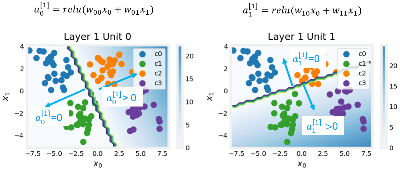
These plots show the function of Units 0 and 1 in the first layer of the network. The inputs are ($x_0,x_1$) on the axis. The output of the unit is represented by the color of the background. This is indicated by the color bar on the right of each graph. Notice that since these units are using a ReLu, the outputs do not necessarily fall between 0 and 1 and in this case are greater than 20 at their peaks.
The contour lines in this graph show the transition point between the output, $a^{[1]}_j$ being zero and non-zero. Recall the graph for a ReLu : The contour line in the graph is the inflection point in the ReLu.
Unit 0 has separated classes 0 and 1 from classes 2 and 3. Points to the left of the line (classes 0 and 1) will output zero, while points to the right will output a value greater than zero.
Unit 1 has separated classes 0 and 2 from classes 1 and 3. Points above the line (classes 0 and 2 ) will output a zero, while points below will output a value greater than zero. Let's see how this works out in the next layer!
Layer 2, the output layer 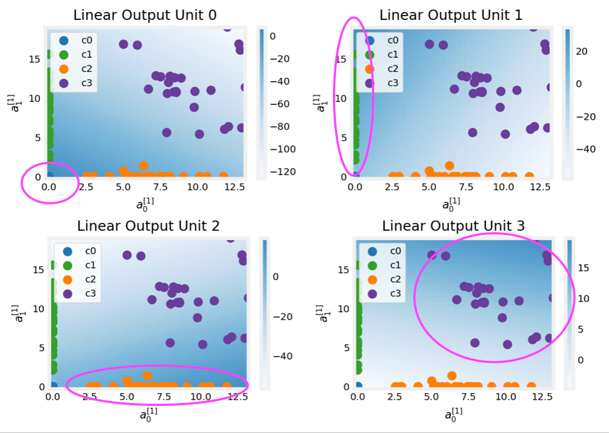
The dots in these graphs are the training examples translated by the first layer. One way to think of this is the first layer has created a new set of features for evaluation by the 2nd layer. The axes in these plots are the outputs of the previous layer $a^{[1]}_0$ and $a^{[1]}_1$. As predicted above, classes 0 and 1 (blue and green) have $a^{[1]}_0 = 0$ while classes 0 and 2 (blue and orange) have $a^{[1]}_1 = 0$.
Once again, the intensity of the background color indicates the highest values.
Unit 0 will produce its maximum value for values near (0,0), where class 0 (blue) has been mapped.
Unit 1 produces its highest values in the upper left corner selecting class 1 (green).
Unit 2 targets the lower right corner where class 2 (orange) resides.
Unit 3 produces its highest values in the upper right selecting our final class (purple).
One other aspect that is not obvious from the graphs is that the values have been coordinated between the units. It is not sufficient for a unit to produce a maximum value for the class it is selecting for, it must also be the highest value of all the units for points in that class. This is done by the implied softmax function that is part of the loss function (SparseCategoricalCrossEntropy). Unlike other activation functions, the softmax works across all the outputs.
You can successfully use neural networks without knowing the details of what each unit is up to. Hopefully, this example has provided some intuition about what is happening under the hood.
Congratulations!
You have learned to build and operate a neural network for multiclass classification.